Week1 - Motivation and Basics
Table of Contents
- Weekly Objectives
- Motivate the study on
- Machinelearning,AI,Datamining….
- Why? What?
- Overview of the field
- Short questions and answers on a story
- What consists of machine learning?
- MLE
- MAP
- Some basics
- Probability
- Distribution
- And some rules…
- Motivate the study on
Maximum Likelihood Estimation
Binomial Distribution
- Binomialdistributionis
- The discrete probability distribution
- Of the number of successes in a sequence of n independent yes/no experiments, and each success has the probability of \(\theta\)
- Also called a Bernoull iexperiment
- Flips are i.i.d
- Independent events (처음 던질 때와 두 번째 던질 때 연관이 없는 상태)
- Identically distributed according to binomial distribution (던질때마다 동일한 확률 분포를 가질 때)
- P(H) = \(\theta\), P(T)=1 - \(\theta\)
- P(HHTHT)= \(\theta \cdot \theta \cdot (1- \theta) \cdot \theta \cdot (1- \theta) = \theta ^3(1 - \theta)^2\)
- Let’s say
- D as Data = H, H, T, H, T
- n = 5
- k = \(a_H\) =3
- p = \(\theta\)
- p(D\(\mid \theta\)) = \(\theta ^{a_H} (1-\theta)^{a_T}\)
- D as Data = H, H, T, H, T
How to get the probability?
Maximum Likelihood Estimation
- p(D\(\mid \theta\)) = \(\theta ^{a_H} (1-\theta)^{a_T}\)
- Data: We have obseved the sequence data of D with \(a_H\) and \(a_T\)
- Our hypothesis:
- The gambiling result follows the binomial distribution of \(\theta\)
- How to make our hypothesis strong(어떻게 ‘참’이다라고 말할 수 있을까)?
- Finding out a better distribution of the observation
- Can be done, but you need more rational.
- Binomial distribution보다 좋은 hypothesis 구조가 있다면, 이것도 가능하지만 더 많은 합리적 생각이 필요.
- Finding out the best candidate of \(\theta\)
- What’s the condition to make \(\theta\) most plausible ?
- \(\theta\)를 최적화하여 hypothesis를 strong하게 만들 수 있음.
- Finding out a better distribution of the observation
어떤 \(\theta\)를 선택했을 때 data를 가장 잘 설명할 수 있을까?
- One candidate is the __Maximum Likelihood Estimation (MLE) of \(\theta\)
- Choose \(\theta\) that maximized the probability of obseverd data
MLE calculation
- \[\hat{\theta} = argmax_\theta P(D| \theta) = argmax_\theta \theta ^{a_H} (1-\theta)^{a_T}\]
- This is going nowhere, so you use a trick (자승을 처리하기 까다로움)
- Using the log function.
- \[\hat{\theta} = argmax_\theta ln P(D| \theta) = argmax_\theta ln(\theta ^{a_H} (1-\theta)^{a_T}) = argmax_\theta ( a_H ln\theta + a_T ln (1-\theta) )\]
- Then, thish is a maximization problem, so you use a derivative that is set to zero
- \[\frac{d}{d\theta} ( a_H ln\theta + a_T ln (1-\theta) ) = 0\]
- \[\frac{a_H}{\theta} - \frac{a_T}{1-\theta} = 0\]
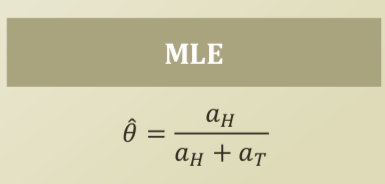
- \[\theta = \frac{a_H}{a_T + a_H}\]
- When \(\theta\) is \(\frac{a_H}{a_T + a_H}\), the \(\theta\) becomes the best candidate from the MLE perspective.
- \[\hat{\theta} = \frac{a_H}{a_H + a_T}\]
Note
압정을 던져 2/5, 3/5 확률이 나오는 것은 아래의 방법을 통해 계산.
binomial distribution, MLE, opmization(derivative).
Number of Trials & Simple Error Bound
- 시도 횟수가 많아 진다면 무엇이 달라질까?
- 똑같은 \(\theta\) 값이 나옴.
- Additional trials reduce the error of our estimation.
- Right now, we have \(\hat{\theta} = \frac{a_H}{a_H + a_T}, N = a_H + a_T\)
- Let’s say \(\theta^*\) is the true parameter of the thumbrack flipping for any error, \(\epsilon > 0\)
- We have a simple upper bound on the probability provided by Hoeffding’s inequality
- Can you calculate the required number of trials, N?
- To obtain \(\epsilon\) = 0.1 with 0.01% case
Note
This is Probably Approximate Correct(PAC) learning
Maximum a Posteriori Estimation
Incorporating Prior Knowledge
- Merge the previous knowledge to my trial
- \[P(\theta|D) = \frac{P(D|\theta)P(\theta)}{P(D)}\]
- Posterior = (Likelihood x Prior Knowledge) / Normalizing Constant
- Already dealt with \(P(D \mid \theta ) = \theta^ {a_H} (1- \theta) ^{a_T}\)
- \(\theta\)라고 가정하고 이러한 data가 관측될 확률.
- \(P(\theta)\) is part of the pror knowledge
- 왜 압정의 앞/뒤가 이런 확률로 나올까?
- 왜 사람이 이렇게 행동할까?
- P(D)는 많이 중요하지 않음
- 사실 \(\theta\)에 대해 관심이 있음.
- 여러번 시도를 해볼 수 있고, 요즘 data가 많음.
- \(P( \theta \mid D)\) : Poseterior
- Then, it is the conclusion influenced by the data and the prior knowledge? Yes, it will be our future prior knowledge!
- 즉, data가 주어졌을 때 \(\theta\)가 사실일 확률을 표현
- \[P(\theta|D) = \frac{P(D|\theta)P(\theta)}{P(D)}\]
More Formula from Bayes Viewpoint
- \[P(\theta|D) \propto P(D|\theta) P(\theta)\]
- \[P(D|\theta) = \theta^{a_H} (1-\theta)^{a_T}\]
- \(P(\theta)\) = ????
- 어떤 distribution(e.g. binomial distribution)에 의존하여 표현해야함.
- 50%, 50% 사전 지식을 그대로 사용 불가.
- 여러 가지 방법이 있으나, 하나의 방법:
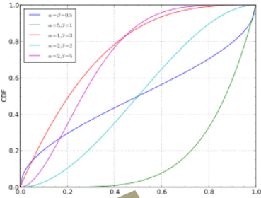
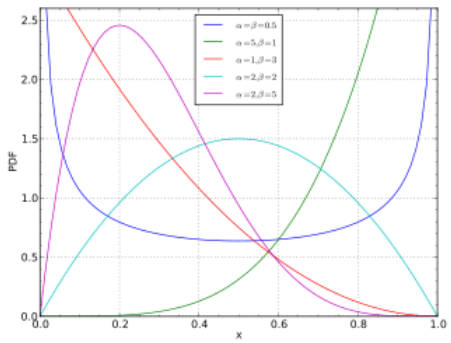
- Beta distribution, 특정범위내에서 [0,1]로 결합되어 있는 CDF로 표현하여 확률 성격을 잘 표현(아래그림참조)
- \[P(\theta) = \frac{\theta ^{\alpha-1} (1-\theta)^{\beta -1 }}{B(\alpha, \beta)}, B(\alpha, \beta) = \frac{\Gamma(\alpha)\Gamma(\beta)}{\Gamma(\alpha+\beta)}, \Gamma (\alpha) = (\alpha -1 )!\]
- Response is
- \[P(\theta) \propto P(D|\theta) P(\theta) \propto \theta ^{a_H} (1-\theta)^{a_T }\theta ^{\alpha-1} (1-\theta)^{\beta -1 } = \theta ^{a_H + \alpha-1} (1-\theta)^{a_T + \beta -1 }\]
Maximum a Posterior Estimation
- Goal: the most probable and more approximate \(\theta\)
- Previously in MLE, we found \(\theta\) from \(\hat{\theta} = argmax_\theta P(D\mid \theta)\)
- \[P(D| \theta) = \theta ^{a_H} (1-\theta)^{a_T }\]
- \[\hat{\theta} = argmax_\theta P(D| \theta)\]
- Now in MAP, we find \(\theta\) from \(\hat{\theta} = argmax_\theta P(\theta \mid D)\)
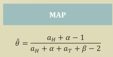
- \[P( \theta|D) \propto \theta ^{a_H + \alpha-1} (1-\theta)^{a_T + \beta -1 }\]
- \[\hat{\theta} = \frac{ \theta ^{a_H + \alpha-1} }{ \theta ^{a_H + \alpha + a_T + \beta -2} }\]
- The calculation is same because anyhow it is the maximization.
Note
Likelihood에 대해 maximization을 하는 것(MLE)이 아니고, posterior에 관하여 maximization(MAP).
Conclusion from Anecdote
- If \(a_H\) and \(a_T\) become big, \(\alpha\) and \(\beta\) becomes nothing..
- But, \(\alpha\) and \(\beta\) are important if I don’t give you more trials.
- \(\alpha\) and \(\beta\)을 선택함에 따라 결과가 달라짐.
Basics
Probability
- Philosophically, Either of the two
- Objectivists assign numbers to describe states of events, i.e. counting
- Subjectivists assign numbers by your own belief to events, i.e. betting
- Mathematically
- A function with the below characteristics
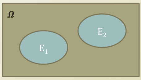
Conditional Probability
- We often do not handle the universe, \(\Omega\)
- Somehow, we always make conditions
- Assuming that the parameters are X, Y, Z, …
- Assuming that the events in the scope of X, Y, Z, …
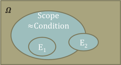
- \[P(A \mid B) = \frac{P(A\cap B)}{P(B)}\]
- The conditional probability of A given B
- Some handy formular
- \[P(B \mid A) = \frac{P(A \mid B) P(B)}{P(A)}\]
- Nice to see that we can switch the condition and the target event
- Poseterior = (Likelihood X Prior Knowledge) / Normalizing Constant
- \[P(A) = \sum_{n} P(A \mid B_n) P(B _n)\]
- Nice to see that we can recover the target event by adding the whole conditional probs and priors
- \[P(B \mid A) = \frac{P(A \mid B) P(B)}{P(A)}\]
Probability Distribution
- Probability distribution assigns
- A probability to a subset of the potential events of a random trial, experiment, survey, etc.
- A function mapping an event to a probability
- Because we call it a probability, the probability should keep its own characteristics(or axiomes)
- An event can be
- A continuous nemeric value from surveys, trials, experiments …
- A discrete categorical value from surveys, trials, experiments …
- For example,
- f: a probability distribution function
- x: a continous value
- f(x): assigned probs \(\begin{aligned} f(x) = \frac{e^{- \frac{1}{2} x^2}}{\sqrt{2 \pi}} \end{aligned}\)
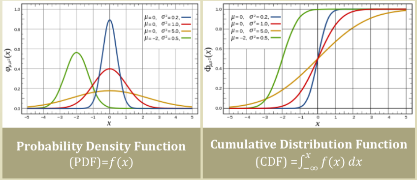
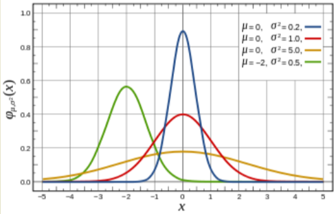
Normal Distribution
- Very commonly observed distribution
- Continuous numerical value
- \[f(x; \mu, \sigma) = \frac{1}{\sigma \sqrt{2\pi}} e ^{- \frac{(x - \mu)^2}{2 \sigma ^2}}\]
- Notation: \(N(\mu, \sigma ^2)\)
- Mean: \(\mu\)
- Variance: \(\sigma^2\)
Beta Distribution
- Supports a closed interval
- Continuous numerical value
- [0,1]
- Very nice characteristic
- Why?
- Matches up the characteristics of probs
- f(\(\theta\); $$\alpha, \beta\() =\)P \frac{\theta ^{\alpha-1} (1-\theta)^{\beta -1 }}{B(\alpha, \beta)}, B(\alpha, \beta) = \frac{\Gamma(\alpha)\Gamma(\beta)}{\Gamma(\alpha+\beta)}, \Gamma (\alpha) = (\alpha -1 )!$$
- Notation: Beta(\(\alpha, \beta\))
- Mean: \(\frac{\alpha}{\alpha + \beta}\)
- Variance: \(\frac{\alpha \beta}{(\alpha + \beta)^2 (\alpha + \beta +1)}\)
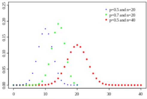
Binomial Distribution
- Simplest distribution for discrete values
- Bernoulli trial, yes or no
- 0 or 1
- Selection, switch …
- \[f(\theta; n, p) = \binom{n}{k} p^k (1-p)^{n-k}, \binom{n}{k} = \frac{n!}{k! (n-k)!}\]
- Notation: \(B(n,p)\)
- Mean: \(np\)
- Variance: \(np(1-p)\)
Multinomial Distribution
- The generalization of the binomial distribution
- e.g., Choose A, B, C, D, E,….,Z
- \[f(x_1, ..., x_k; n, p_1, ..., p_k) = \frac{n!}{x_1! ... x_k !} p_1^{x_1} \cdot p_k^{x_k}\]
- Notation: Multi(P), \(P=< p_1, ..., p_k>\)
- Mean: \(E(x_i) = np_i\)
- Variance: Var\((x_i) = np_i (1-p_i)\)
Summary
압정 던지는 시도를 통해서 다음번에 무엇이 나올 지 확률을 계산하는 것은 단순히 (횟수/시도) 되는 것이 아니라, 이항분포 가정-> MLE or MAP(사전지식이용) -> optimization(derivative) 과정을 통해 도출되는 것임을 이해했다.
MAP는 likelihood를 최대화 하는 MLE 과정에 추가적으로 사전 지식을 사용하기 위해 베이즈 룰을 이용하여 posteriori를 계산하는데 적용이 되었으며, 사전 지식은 Beta 분포(0~1 범위를 가지는 연속분포)라고 가정하여 계산할 수 있었다.
- 그러나, 결과적으로 시도 횟수가 많아 지게 되면 MLE, MAP는 동일한 결과를 얻을 수 있다.
Reference: