Robot Dynamics & control: Lecture 3 - Forward Kinematics: The Denavit-Hartenberg Convention
in Robotics / Robotics & Control on Robotics
Table of Contents
Introduction
- The forward kinematics problem is to determine the position and orientation of the end-effector, given the values for the joint variables of the robot.
- The joint variables: angle between the links for revolute or rotational joint link extension for the prismatic or sliding joint.
- \(f\): forward kinematics
Kinematic Chains
- A robot manupulator n joints will have n+1 links including ground.
- Joint number: 1 ~ n, Link number: 0 ~ n
- Joint i connects link i-1 to link i.
- Joint i is fixed at link i-1, so when joint i is actuated, link i moves.
- Link 0(the first link) is fixed and does not move when the joints are actuated.
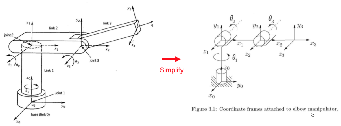
- With the i^{th} joint, we associate a joint variable, denoted by q_i.
- \(\theta_i\): joint \(i\) revolute
- \(d_i\): joint \(i\) prismatic
- \(o_i x_i y_i z_i\) is attached to link i \(\rightarrow\) when joint i is actuated, link i and its attached frame \(o_i x_i y_i z_i\) experience a resulting motion.
- The frame \(o_0 x_0 y_0 z_0\) which is attached to the robot base, is referred to as the inertial frame(=world coordinate).
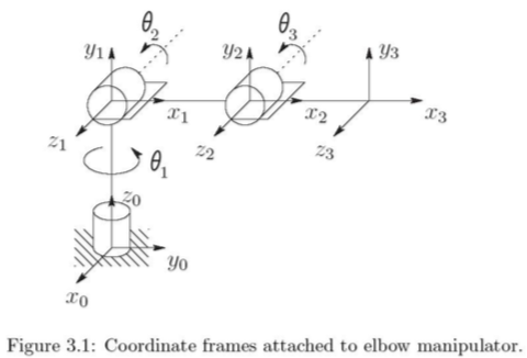
- Suppose \(A_i\) is the homogeneous transformation matrix that expresses the position and orientation of \(o_i x_i y_i z_i\) with respect to \(o_{i-1} x_{i-1} y_{i-1} z_{i-1}\).
- The matrix \(A_i\) is not constant but varies as the configuration of the robot is changed, and \(A_i\) is a function of only a single joint variable, namely \(q_i\).
- Homogeneous transformation matrix \(T^i_j\) that expresses the position and orientation of \(o_j x_j y_j z_j\) with respect to \(o_i x_i y_i z_i\) .
- The homogeneous transformation matrix denoted by the position(\(o^0_n\)) and orientation (\(R^0_n\)) of the end-effector with respect to the inertial or base frame:
- This is forward kinematics!
- But, it is possible to achieve a considerable amount of stream linking and simplication by introducing D-H representation.
- Each homogeneous transformation matrix:
- Hence,
- It is possible to carry out all of the analysis using an arbitrary frame attached to each link.
- However, it is helpful to be systematic in the choice of these frames by using the Denavit-Hartenberg, or D-H convention.
- In D-H convention, each homogeneous tranformation matrix \(A_i\) is represented as a product of four basic transformations.
Denavit - Hartenberg Representation
\[\begin{aligned} A &= Rot_{z, \theta_i} Trans_{z, d_i} Trans_{x, a_i} Rot_{x, \alpha_i} \\ &= \begin{bmatrix} c_{\theta_i} & -s_{\theta_i} & 0 & 0\\ s_{\theta_i} & c_{\theta_i} & 0 & 0\\ 0 & 0 & 1 & 0\\ 0 & 0 & 0 & 1\\ \end{bmatrix} \begin{bmatrix} 1 & 0 & 0 & 0\\ 0 & 1 & 0 & 0\\ 0 & 0 & 1 & d_i\\ 0 & 0 & 0 & 1\\ \end{bmatrix} \begin{bmatrix} 1 & 0 & 0 & a_i\\ 0 & 1 & 0 & 0\\ 0 & 0 & 1 & 0\\ 0 & 0 & 0 & 1\\ \end{bmatrix} \begin{bmatrix} 1 & 0 & 0 & 0\\ 0 & c_{\alpha_i} & - s_{\alpha_i}& 0\\ 0 & s_{\alpha_i} & c_{\alpha_i}& 0\\ 0 & 0 & 0 & 1\\ \end{bmatrix} \\ &= \begin{bmatrix} c_{\theta_i} & -s_{\theta_i}c_{\alpha_i} & s_{\theta_i}s_{\alpha_i} & \alpha_i c_{\theta_i}\\ s_{\theta_i} & c_{\theta_i}c_{\alpha_i} & -c_{\theta_i}s_{\alpha_i} & \alpha_i s_{\theta_i}\\ 0 & s_{\alpha_i} & c_{\alpha_i}& d_i\\ 0 & 0 & 0 & 1\\ \end{bmatrix} \end{aligned}\]- Since the matrix A_i is a function of a single variable, the 3 of the 4 quantities are constant for a given link.
- \(d_i\): Joint variable for a prismatic joint.
- \(\theta_i\): Joint variable for a revolute joint.
By a clever choice of the origin and coordinate axes, it is possible to cut down the number of parameters and needed from 6 to 4.
- Existence and uniqueness issues:
- Clearly, it is not possible to represent any arbitrary homogeneous transformation using only four parameters
- But, is is possible to derive a unique homogeneous transformation matrix \(A\) under the following two conditions.
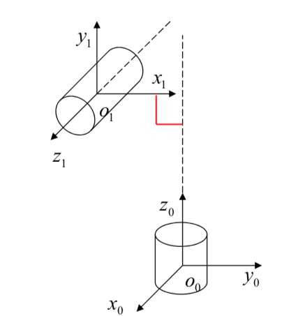
DH1) The axis \(x_1\) is perpendicular to the axis \(z_0\).
DH2) The axis \(x_1\) intersects the axis \(z_0\)
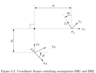
- Under DH1 and DH2, we claim that there exist unique numbers \(a, d, \theta , \alpha\) such that.
- \[A = Rot_{z,\theta} Trans_{z,d} Trans_{x,a} Rot_{x, \alpha}\]
- Physical interpretation of four quantities:
- a: Distance between the axes \(z_0\) and \(z_1\) measured along the axis \(x_1\)
- d: Distance between the origin \(o_0\) and the intersection of the \(x_1\) axis with \(z_0\) measured along the \(z_0\) axis.

- Physical interpretation of 4 quantities:
- \(\alpha\): Angle between the axes \(z_0\) and \(z_1\) measured in a plane normal to \(x_1\).
- \(\theta\): Angle between \(x_0\) and \(x_1\) measured in a plane normal to \(z_0\).
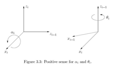
- Assigning the coordinate frames
- For a given robot manipulator, one can always choose the frame 0, 1, …, n in such a way that the DH1 and DH2 are satisfied.
- It is important to keep in mind that the choices of the various coordinate frames are not unique, even when constrained by the DH1 and DH2.
- However, it is important to note that the end result(\(T^0_n\)) will be the same, regardless of the assignment if untermediate link frames .
- We assign \(z_i\) to be the axis of actuation for joint i+1
- If joint i+1 is revolute, \(z_i\) is the axis of revolution of joint i+1.
- If joint i+1 is prismatic, \(z_i\) is the axis of translation of joint i+1.
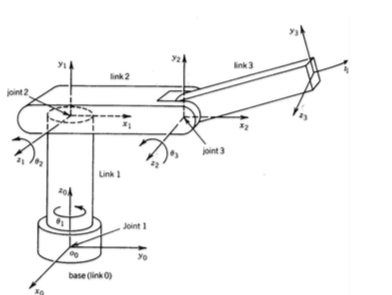
- In order to set up frame i it is necessary to consider 3 cases:
- case 1:
- \(z_{i-1}\) and \(z_i\) are not coplanar:
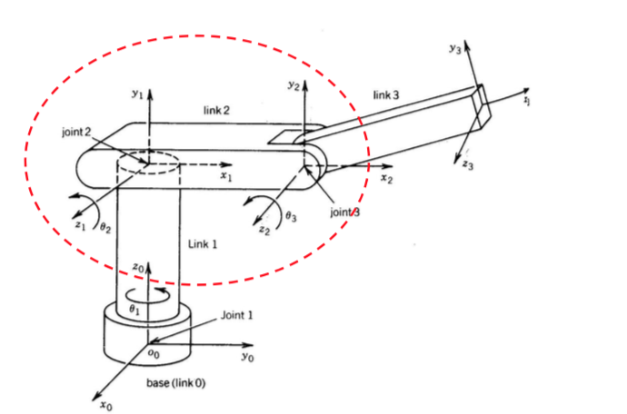
- case 2:
- \(z_{i-1}\) is parallel to \(z_i\):
- \(d_i, \alpha_i\) are 0 in this case
- \(z_{i-1}\) is parallel to \(z_i\):
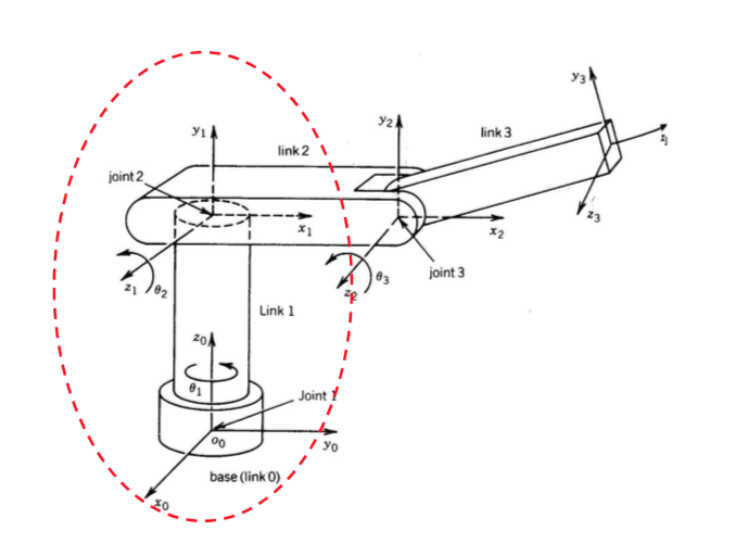
- case 3:
- \(z_{i-1}\) intersects \(z_i\):
- \(a_i\) are 0 in this case
- \(z_{i-1}\) intersects \(z_i\):
- This constructive procedure works frame 0, …, n-1 in an n-link robot.
- The final coordinate system \(o_n x_n y_n z_n\) is commonly referred to as the end-effctor(or tool frame)
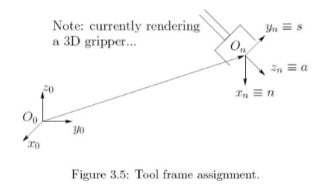
Terminology arises from the fact that the direction a is the approach direction, the s direction is the sliding direction, and n is the direction normal to the plane formed by a and s.
- Note the following important fact:
- The quantities \(a_i\) and \(\alpha\) are always constant (characteristics of the manipulator)
- If joint i is prismatic, then \(\theta_i\) is also a constant, while \(d_i\) is the \(i^{th}\) joint variable.
- If joint i is revolute, then \(d_i\) is also a constant, while \(\theta_i\) is the \(i^{th}\) joint variable.
- Summary:
\(1.\) Locate and label the joint axes \(z_0, ..., z_{n-1}\).
\(2.\) Establish the base frame. Set the origin anywhere on the \(z_0\)-axis. The \(x_0\) and \(y_0\) axed are chosen conveniently to form a right-hand frame. For i = 1, …, n-1, perform step 3 to 5.
\(3.\) If \(z_i\) intersects \(z_{i-1}\), locate \(o_i\) at this intersection. If \(z_i\) and \(z_{i-1}\) are parallel, locate \(o_i\) in any convenient position along \(z_i\).
\(4.\) Establish \(x_i\) along the common normal between \(z_{i-1}\) and \(z_i\) through \(o_i\), or in the direction normal to the \(z_{i-1} - z_i\) plane if \(z_{i-1}\) and \(z_i\) intersect.
\(5.\) Establish \(y_i\) to complete a right-hand frame
\(6.\) Establish the end-effector frame \(o_n x_n y_n z_n\). Assuming the n-th joint is revolute, set \(z_n\) = a along the direction \(z_{n-1}\). Establish the origin on conveniently along \(z_n\), preferably at the center of the gripper or at the tip of any tool. Set \(y_n\) = s in the direction of the gripper closure.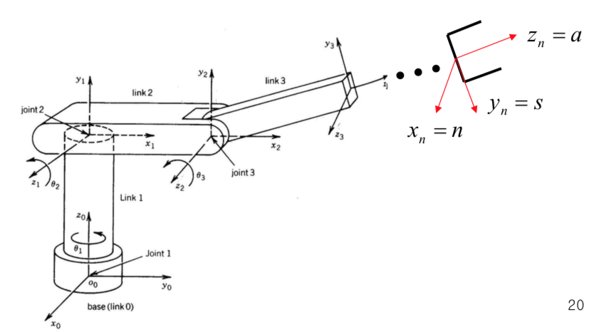
\(7.\) Create a table of link parameters \(a_i, \alpha_i , d_i, \theta_i\).
\(8.\) From the homogeneous transformation matrices \(A_i\) by substituting the above parameters into \[\begin{aligned} A &= Rot_{z, \theta_i} Trans_{z, d_i} Trans_{x, a_i} Rot_{x, \alpha_i} \\ &= \begin{bmatrix} c_{\theta_i} & -s_{\theta_i}c_{\alpha_i} & s_{\theta_i}s_{\alpha_i} & \alpha_i c_{\theta_i}\\ s_{\theta_i} & c_{\theta_i}c_{\alpha_i} & -c_{\theta_i}s_{\alpha_i} & \alpha_i s_{\theta_i}\\ 0 & s_{\alpha_i} & c_{\alpha_i}& d_i\\ 0 & 0 & 0 & 1\\ \end{bmatrix} \end{aligned}\]
\(9.\) Form \(T^0_n = A_1 \cdots A_n\). This then gives the position and orientation of the tool frame expressed in base coordinates.
Reference: